Quick Navigation
- 1How Excel Stores Dates
- 2How Excel Stores Times
- 3Working with Dates and Times
- 3.1DATE() and TIME()
- 4Additional Date and Time Setting Functions
- 4.1TODAY()
- 4.2NOW()
- 4.3EDATE() and EOMONTH()
- 4.4WORKDAY()
- 4.5WORKDAY.INTL() (Excel 2010 and newer)
- 5Retrieving Dates in Excel
- 5.1DAY(), MONTH(), and YEAR()
- 6Retrieving Times in Excel
- 6.1HOUR(), MINUTE(), and SECOND()
- 7Additional Date Retrieving Functions
- 7.1WEEKDAY() and WEEKNUM()
- 8Counting and Tracking Dates
- 8.1NETWORKDAYS()
- 8.2NETWORKDAYS.INTL() (Excel 2010 and newer)
- 8.3YEARFRAC()
- 8.4DATEDIF() (Undocumented Function)
- 9Converting Dates and Times from Text
- 9.1DATEVALUE() and TIMEVALUE()
- 10Converting Dates and Times to Text
- 10.1TEXT()
- 11A Common Problem
 Dates and times are two of the most common data types people work with in Excel, but they are also possibly the most frustrating to work with, especially if you are new to Excel and still learning. This is because Excel uses a serial number to represent the date instead of a proper month, day, or year, nevermind hours, minutes, or seconds. It’s made more complicated by the fact that dates are also days of the week, like Monday or Friday, even though Excel doesn’t explicitly store that information in the cells. Here is the definitive guide to working with dates and times in Excel…
How Excel Stores Dates
The source of most of the confusion around dates and times in Excel comes from the way that the program stores the information. You’d expect it to remember the month, the day, and the year for dates, but that’s not how it works…
Excel stores dates as a serial number that represents the number of days that have taken place since the beginning of the year 1900. This means that January 1, 1900 is really just a 1. January 2, 1900 is 2. By the time we get all the way to the present decade, the numbers have gotten pretty big… September 10, 2013 is stored as 41527.
Importantly, any date before January 1, 1900 is not recognized as a date in Excel. There are no “negative” date serial numbers on the number line.
It seems confusing, but it makes it a lot easier to add, subtract, and count days. A week from September 10, 2013 (September 17, 2013), is just 41527 + 7 days, or 41534.
How Excel Stores Times
Excel stores times using the exact same serial numbering format as with dates. Days start at midnight (12:00am or 0:00 hours). Since each hour is 1/24 of a day, it is represented as that decimal value: 0.041666…
That means that 9:00am (09:00 hours) on September 10, 2013 will be stored as 41527.375.
When a time is specified without a date, Excel stores it as if it occurred on January 0, 1900. In other words, 3:00pm (15:00 hours) is stored as 0.625. This can make doing math for time-only values (that have no date) challenging, since subtracting 6 hours (6:00) from 3:00am (03:00 hours) will become negative and count as an error: 0.125 – 0.25 = -0.125, which is displayed as #########.
Minutes and seconds in Excel work the same way as hours…
A minute is 1/60 of an hour, which is 1/24 of a day, or 1/1440 of a day in total, which calculates to 0.00069444…
A second is 1/60 of an minute, which is 1/60 of an hour, which is 1/24 of a day, or 1/86400 of a day in total, which calculates to 0.00001157407…
Working with Dates and Times
DATE() and TIME()
Serial numbers aren’t all that intuitive to use. Fortunately, Excel has a set of functions to make it easier to find and use dates and times, starting with DATE and TIME. The syntax is as follows:
=DATE(year, month, day)
=TIME(hours, minutes, seconds)
For both functions, specify the year, month, and day, or hours, minutes, and seconds as numbers. For example, September 10, 2013 can be entered as:
=DATE(2013,9,10)
It will be stored as 41527, which means that it is technically storing 12:00am on September 10, 2013.
For times, 6:00pm (18:00 hours) can be entered as:
=TIME(18,0,0)
It will be stored as 0.75, which means that it is technically storing 6:00pm on January 0, 1900.
If we want to represent a specific time and date, we can add the two functions together. For example, 6:00pm (18:00 hours) on September 10, 2013 can be entered as:
=DATE(2013,9,10)+TIME(18,0,0)
It will be calculate as 41527.75, which means Excel is storing exactly the date we want…
Additional Date and Time Setting Functions
Excel has a few additional functions to make declaring dates easier.
TODAY()
The TODAY function always returns the current date’s serial number. The TODAY function is just entered as:
=TODAY()
This article was written at 6:30pm (18:30 hours) on September 24, 2013, and the TODAY function calculated to 41541. That means that it is technically storing 12:00am on September 24, 2013.
NOW()
A similar function called NOW always returns the current date and time’s serial number. The NOW function is just entered as:
=NOW()
Again, at 6:30pm (18:30 hours) on September 24, 2013, the function calculated to 41541.77081333… NOW stores the exact time and date, down to the second.
EDATE() and EOMONTH()
The EDATE function gives the date the specified number of months away from the input date. The EOMONTH function gives the date of the last day of the month. It can do so for the current month or a number of months in the future or the past. The syntax for each is as follows:
=EDATE(start_date, months)
=EOMONTH(start_date, months)
The start_date can be any date-formatted cell reference or date serial number.
The months field can be any number, though only the integer value will be used (e.g. it treats 2.8 as 2).
The EDATE and EOMONTH functions strip the time value from the date. For example, For example, if cell A1 stores September 10, 2013, we can get the value 2 months ahead as follows:
=EDATE(A1,2)
Returns 12:00am (0:00 hours) on November 10, 2013, or 41588. This function works even though the months have different numbers of days (September and November have 30, October has 31).
=EOMONTH(A1,2)
Returns 12:00am (0:00 hours) on November 30, 2013, or 41588. Again, this function works even though the months have different numbers of days.
WORKDAY()
Occasionally, it may be useful to count ahead based on work-days (Monday-Friday) instead of all 7 days of the week… For that, Excel has provided WORKDAY. The syntax for WORKDAY is as follows:
=WORKDAY(start_date, days, [holidays])
The start_date is as above.
The days input is the number of workdays ahead (or behind) of the present day you would like to move.
The [holidays] input is optional, but lets you disqualify specific days (like Thanksgiving or Christmas, for example), which might otherwise fall during the work week. These are date serial numbers provided in an array bounded by brackets: { }. To specify multiple holidays, the dates must be held in cells – it is not possible to put multiple DATE functions in an array.
For example, let’s find the date 6 work days before 6:00pm (18:00 hours) on September 10, 2013 (stored in cell A1). Monday, September 2nd is Labor Day, so let’s include that as a holiday:
=WORKDAY(A1,-6,DATE(2013,9,2))
Returns 12:00am (0:00 hours) on August 30, 2013, or 41516. (Note that the function strips the time portion of the date.)
WORKDAY.INTL() (Excel 2010 and newer)
For newer versions of Excel (2010 and later), there is another version of WORKDAY called WORKDAY.INTL. WORKDAY.INTL works just like WORKDAY, but it adds the ability to customize the definition of the “weekend”. The syntax for WORKDAY.INTL is as follows:
=WORKDAY.INTL(start_date, days, [weekend], [holidays])
The start_date, days, and [holidays] inputs work just like the normal WORKDAY function.
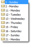
The [weekend] input has the following options:
Retrieving Dates in Excel
DAY(), MONTH(), and YEAR()
Now we know how define dates, but we still need to be able to work with them. Serial numbers don’t make it easy to extract months, years, and days, nevermind hours, minutes, and seconds. That’s why Excel has specific functions for pulling out each of these values. For working with the calendar, there is DAY, MONTH, and YEAR. The syntax is simple:
=DAY(serial_number)
=MONTH(serial_number)
=YEAR(serial_number)
The serial_number in each can be any date-formatted cell reference. For example, if cell A1 stores September 10, 2013, we can use each of the formulas in turn:
=DAY(A1)
Returns 10 as a numeric value.
=MONTH(A1)
Returns 9 as a numeric value.
=YEAR(A1)
Returns 2013 as a numeric value.
We could have also given the direct serial number for September 10, 2013:
=DAY(41527)
Returns 10 as a numeric value.
Retrieving Times in Excel
HOUR(), MINUTE(), and SECOND()
For times, the process is very similar. Excel has function to retrieve the hours, minutes, and seconds from a time stamp, conveniently named HOUR, MINUTE, and SECOND. The syntax is identical:
=HOUR(serial_number)
=MINUTE(serial_number)
=SECOND(serial_number)
The serial_number in each can be any time/date-formatted cell reference. For example, if A1 stores 6:15:30pm (18:15 hours, 30 seconds) on September 10, 2013, we can use each of the formulas in turn:
=HOUR(A1)
Returns 18 as a numeric value.
=MINUTE(A1)
Returns 15 as a numeric value.
=SECOND(A1)
Returns 30 as a numeric value.
We could have also given the direct serial number for 6:15:30pm (18:15 hours, 30 seconds) on September 10, 2013:
=SECOND(41527.7607638889)
Returns 30 as a numeric value.
Additional Date Retrieving Functions
WEEKDAY() and WEEKNUM()
Dates don’t just have month and year information. They also encode indirect information… September 10, 2013 happens to also be a Tuesday. Excel has a few of functions to work with the week aspect of dates: WEEKDAY and WEEKNUM. The syntax is as follows:
=WEEKDAY(serial_number, [return_type])
=WEEKNUM(serial_number, [return_type])
The serial_number in each can be any date-formatted cell reference. Since [return_type] is optional, each function assumes that each week starts on Sunday. If cell A1 stores September 10, 2013 (a Tuesday), we can use each of the formulas in turn:
=WEEKDAY(A1)
Returns 3, since Tuesday is the 3rd day of a week that starts on Sunday.
=WEEKNUM(A1)
Returns 37, since September 10, 2013 is in the 37th week of 2013, when you start counting weeks from Sunday.
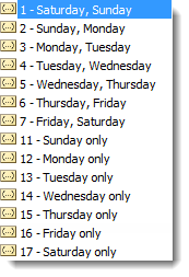
The [return_type] allows you to specify a different default week arrangement. You could let the week start on Monday and run until Sunday, or Saturday until Friday, for example. Excel is annoying, however, and makes the entry different for WEEKDAY and WEEKNUM. The full list of options for WEEKDAY is as follows:
Options 2 and 11 are functionally the same – the first is just there for backwards compatibility with earlier versions of Excel.
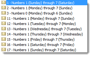
The full list of options for WEEKNUM is as follows:
Counting and Tracking Dates
Dates can be added and subtracted like normal numbers because they’re stored as serial numbers. That lets you count the days between two different dates. Sometimes, though, you need to count by a different metric.
NETWORKDAYS()
Above, we learned about WORKDAY, which lets you move back and forth a set number of workdays, ignoring weekends and holidays. But what if you need to measure the number of workdays between two dates? For that, Excel provides NETWORKDAYS. The formula syntax is as follows:
=NETWORKDAYS(start_date, end_date, [holidays])
The start_date and end_date can be any date-formatted cell reference.
The [holidays] input is optional, but lets you disqualify specific days (like Thanksgiving or Christmas, for example), which might otherwise fall during the work week. These are date serial numbers provided in an array bounded by brackets: { }. To specify multiple holidays, the dates must be held in cells – it is not possible to put multiple DATE functions in an array.
For example, if A1 contains 6:00pm (18:00 hours) on September 10, 2013 and B1 contains 9:00am (9:00 hours) on December 2, 2013, we can use NETWORKDAYS to find the number of workdays between the two dates.
Let’s exclude Columbus Day (October 14, 2013), Veterans Day (November 11, 2013), and Thanksgiving Day (November 28, 2013) as holidays. To do so, we have to store those dates in other cells. Let’s put them in C1, C2, and C3:
=DATE(2013,10,14)
=DATE(2013,11,11)
=DATE(2013,11,28)
Now, we can combine them in the function:
=NETWORKDAYS(A1,B1,C1:C3)
The function returns 57 as a numeric value.
NETWORKDAYS.INTL() (Excel 2010 and newer)
For newer versions of Excel (2010 and later), there is another version of NETWORKDAYS called NETWORKDAYS.INTL. NETWORKDAYS.INTL works just like NETWORKDAYS, but it adds the ability to customize the definition of the “weekend”. The syntax for NETWORKDAYS.INTL is as follows:
=NETWORKDAYS.INTL(start_date, end_date, [weekend], [holidays])
The start_date, end_date, and [holidays] inputs work just like the normal WORKDAY function.
The [weekend] input has the following options:
YEARFRAC()
Sometimes it’s useful to measure how much time has passed in years, but subtracting the YEAR function will only round down to the nearest full year. YEARFRAC takes two dates and provides the portion of the year between them. The syntax is as follows:
=YEARFRAC(start_date, end_date, [basis])
The start_date and end_date can be any date-formatted cell reference.
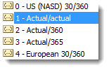
The [basis] input is optional, but lets you specify the “rules” for measuring the difference. Most of the time, you’ll want to use option 1, but here is the full list:
 For example, if A1 contains September 10, 2013 and B1 contains December 2, 2013, we can use YEARFRAC to find the decimal portion of a year between the two dates:
=YEARFRAC(A1,B1,1)
Returns 0.227397260273973.
DATEDIF() (Undocumented Function)
The YEARFRAC function gives you the difference between dates as a fraction of a year, but sometimes you need more control. There is a powerful hidden function in Excel called DATEDIF that can do much more. It can tell you the number of years, months, or days between two dates. It can also track based on only partial inputs, ignoring years or months when calculating days. The syntax for DATEDIF is as follows:
=DATEDIF(start_date, end_date, unit)
The start_date and end_date can be any date-formatted cell reference.
The unit input asks you to specify a string that represents the type of output you want. This is slightly cumbersome, since you must wrap the input in quotes (” “).
For example, if A1 contains September 10, 2012 and B1 contains December 2, 2013, we can use DATEDIF to find the number of full years between the two dates:
=DATEDIF(A1,B1,"Y")
Returns 1 as a numeric value.
Using the same start_date and end_date inputs, here are the output possibilities for DATEDIF using different unit parameters:
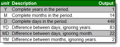
Every time, the unit must be put in quotes (e.g. “Y” or “MD”).
Converting Dates and Times from Text
DATEVALUE() and TIMEVALUE()
All of the above functions work perfectly with date-formatted serial numbers in Excel. Unfortunately, dates and times are often imported into worksheets as text. Most of the assorted functions like MONTH and HOUR are reasonably intelligent about converting on the fly. Occasionally it’s useful to build a date value through concatenation. The two functions Excel provides for this purpose are DATEVALUE and TIMEVALUE. The syntax for each is as follows:
=DATEVALUE(date_text)
=TIMEVALUE(time_text)
The date_text and time_text accept any text string that looks like a date or time.
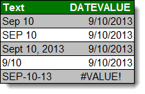
This is how DATEVALUE responds to various date_text inputs:
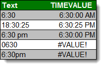
This is how TIMEVALUE responds to various time_text inputs:
Converting Dates and Times to Text
TEXT()
Getting data converted to dates and times is great, but you may also need to get it back out. Sometimes, you need a special format. Other times, you need to look for a date in a text string, and have to match using string tools like FIND and SEARCH. There is one master function for converting dates and times to text strings in Excel, called TEXT. The syntax for TEXT is as follows:
=TEXT(value, format_text)
The value can be any date or time-formatted cell reference.
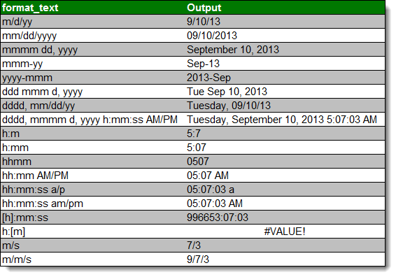
The format_text input has a large number of options, summarized here:
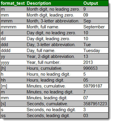
The outputs can be combined with simple formatting characters to produce standard date formats. Using the date 5:07:03am (05:07 hours, 3 seconds) on September 10, 2013, here are examples of possible outputs:
A Common Problem
One issue people frequently run into is that Excel occasionally misinterprets text fields as dates. An example is here:
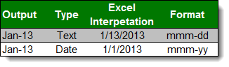
Be careful when entering dates, especially if you are importing from other data sources, to make sure that your “Jan-13” is being stored as January 1, 2013 and not January 13, 2013!
Nice article, very comprehensive. One thing though: If anyone is having the same trouble that I had when using
TEXT(A1,"mmm")then try to use capital letters for the format :TEXT(A1,"MMM"). When I used the version with the lower-case format then the abbreviated month name was displayed as “00”, not as “Jan”, “Feb” etc.THANK YOU1111
Been fighting with this for hours. Found out it actually takes the “mm” for minutes for some reason. In my example I tried to re-create a text string like 19.09.2013 by doing text(C4;”dd.mm.yyyy”) and got 19.00.2013 back! Then I checked and confirmed that the 00 corresponded to minutes, found this article and finally your comment.
Thanks again, hope my point helps Excel to correct this bug
Cheers
I’m trying to add 72 hours to a date/time cell. I can’t add 3 days instead of 72 hours (e.g.) “=A1+3” because the results have to be to the hour. If I do “A1+TIME(72) the result is the same, i.e. it doesn’t change the date. For example, in cell A1 the date/time value is “4/1/2014 6:40:00 AM” and the serial value is “41730.2777777778” . The formula in cell B1 is “=A1+TIME(72,0,0)” but the resulting date/time value is still “4/1/2014 6:40:00 AM” and the serial value is still “41730.2777777778”. Any ideas on how to formulate B1 so the result will be “4/4/2014 6:40:00 AM”?
Hi Stan,
Great question! The TIME() function in Excel truncates the days added, so when you enter more hours than there are in one day it gives you the partial-day remainder (e.g. TIME(30,0,0) will return 0.25 or 6:00 AM).
It sounds like you have an input that will be in terms of hours (since you must enter “72 hours” and not “3 days”). In this case, I suggest you take advantage of Excel’s date storage method and divide your hours by 24 to get the value in days.
In your example, the formula in B1 would be:
=A1+(72/24)If your input is in another cell (let’s assume the 72 is coming from A2), the formula in B1 would be:
=A1+(A2/24)Good luck!
Andrew
Thank you, Andrew. That did the trick. Works great!
Stan
Hello. Thanks for posting this. The issue I’m having is with the 24 vs. 12 hour clock. For example, if in column A I have a series of times, and I use the formula =TEXT(A1, “h:mm”) to return a text value in column B, then for the example of 8:00 PM, the formula yields 20:00. How can I convert this to a 12 hour clock, yielding the result 8:00? Thanks for any suggestions.
Hi Erin,
Great question! To force Excel to use a 12-hour time notation, you must specify the AM/PM element. In your case, the format would be:
=TEXT(A1,"h:mm AM/PM")Good luck!
Andrew
Hi Andrew,
Thanks for the quick response. The formula you provided yields 8:00 PM, but I need to omit the “PM”. Any further suggestions?
Thanks in advance!
It isn’t elegant, but you can remove the AM/PM from this notation by chopping it off:
=LEFT(TEXT(A1,"h:mm AM/PM"),LEN(TEXT(A1,"h:mm AM/PM"))-3)What this does is take the characters to the left of the AM/PM with LEFT(). It figures out where they are by measuring the length of the string with LEN() and subtracting the last 3 (AM or PM plus a space character).
It may not be pretty, but it works, and that’s all that matters 🙂 Thanks so much!
I am importing my pdf bank statements into excel 2010. The dates for each transaction only includes the day and month. Is there an easy way to fill the date column with the year?
Sounds like you’re looking for the DATE() function…
I want Excel to give me the date (day/month) based on the number of days (that have passed in a year). E.g., “54” would result in 23/Feb. Any idea how to do this?
Forget it, just found it. Just “start date + number of days” in date format, so “=1/1/12+G17”.
Thanks anyway 🙂
I have a column of various dates of which I want to add another column of various months to. CANNOT FIGURE IT OUT!
Here is what I’m trying to figure out:
Today’s Date 1: 10/7/14
Date 2 (Due Date): 10/31/14
I would like Excel to look at these two dates, subtract the two (which then is a numerical value), then output “Yes” IF the answer is less than say 90 days.
use this
=IF(DATEDIF(start_date,end_date,”yd”)<90,"yes","")
I have numerous columns of date information (8,000 responses) that came from multiple sources, which I want to standardize.
In a year field, folks responded with (or provided) an odd collection of date formats: 6/92, 06/92, 6/1/1992, 1992, N/A, along with no answer at all. When I use the =YEAR(A2) function to convert the column to year, all varieties of dates that have a “/” in them convert correctly to year. However, “year only” original values convert to 1905, blanks convert to 1900, and N/As convert to #VALUE! Any ideas?
Corollary: In another column, I asked for date and folks responded with the same assortment–what algorithm will convert their mm/yy or m/yyyy to 06/01/1992 or their yy or yyyy to 01/01/1992?
I am trying to create a list of dates to display, but exclude all dates that are a Sunday. So for example, create a list for the year (from today) and list them on excel, but not include any dates in the list that is a Sunday. We work for example Mon-Sat.
Hi,
i am trying to ask excel to automatically enter the month… but i want it to display the name only of the last month… so if today is october 22nd i want my cell to say ‘September’, so then for example when we move into november, i want my cell to say ‘October’ – is there a way to do this?
Thanks
I am trying to track the time is has taken to do a task over two days but only calculating working hours. For instance how long it has taken for me to do something starting at 15.30 on 9th October 2014 and finished 10.45 10th October. I don’t know how to exclude weekends and holidays and over night? Need some help!
Whats the formula or what can we do to stay the informationt type on that date.
Like I put my to do list on the 28 and when i go to next date, it shows the 28 to do list and i only want it to show on 28 and does not follow to 29th.
I am trying to get Excel to see if a manually entered date in the format of “mm/dd/yyyy HH:MM:SS AM” is greater than or equal to a column from a data source that contains data in the following format “mm/dd/yyyy HH:MM:SS AM” and not having much luck.
The input sheet contains the manually enter start date range and end date range of the data you want to examine.
The source sheet contains a data dump from a BMC product and the column contains data in the format of “mm/dd/yyyy HH:MM:SS AM”. (In all of the above mm and dd could be 1 digit or two).
The formula I am trying to use to see if the data falls in between start and end date is listed below.
=IF(AND(G2=”Closed”,’Sheet 1′!E2=Instructions!$D$6),1,”Out of rangeZZZ”)
The result showing false when the source date is really between the start and end dates, and I believe this is because Excel is not treating the manually enter “instructions” sheet date the same as the “Sheet 1” sheet which is the source data.
The Instructions sheet, you manually enter the start and end date/time you want to use for the data range. If the date on the source sheet falls between that range then I want ot place a 1 in a column to sum up later.
Any help would be appreciated.
Thanks
I’m trying to put a log together with over 300 people. so in 1 day I enter their name and I want to show the date and time. i’m entering 100 different items a day. I want the date to just auto fill. how should I do this??
I am copying and pasting a series of data into excel. One of the fields is a project number with the value 15642am. Excel keep converting it to a time becuase it ends in am. How can I trick EXCEL into keeping the field 15642am not 10/12/1901 6:00:00 PM. I tried formatting the column as text before pasting values. I tried formatting the column as text and coping match destination formatting. Niether worked. Any help would be breatly appreciated.
Hi, I was trying to create formula in which excel would look for the Fridays date for that criteria, is that possible?
Here is what I have so far, but its wrong:
=IF(Sheet1!A:A=”ALL”,(MAX(WEEKDAY(Sheet1!B:B, 5))),”WRONG FIX FORMULA”)
so if column A is equal to ALL, then populate this cell with the latest Friday date in column B corresonding to column A.
The date is formulated in (MM/DD/YY HH:MM:SS AM/PM). Column B returns dates not always Monday-Sunday. I just want to latest friday
Not sure if this makes any sense lol.
Hi I am trying to figure out what formula(s) to use in order to make one cell count how many days another cell has been at that value. EX. if A2 shows “N” B2 shows nothing, but if I change A2 to show “Y” I would like B2 to start counting days “1”, “2”.”3″, …
Thank you for any help.
Hi I am trying to figure how to extract the weekends from my today formula
I have =today()+8 for example, so if today starts with a monday, I want this to have a result of a thrursday of next week, other than it being a Tues of next week.
Please help?!
I am trying to use the & command to combine a few cells and the date cell changes to the number value.
from 24-11-2014 to 29-11-2014 using & it comes up as from41967to41972
Hi,
I have a formula set up which essentially adds 7 days on from the inputted date in another cell. For example, if in E1 I input 10/10/14, G1 would automatically fill 17/10/14. This works fine, but my problem is I have a lot of blank rows which won’t have entries until the spreadsheet becomes active. But where there isn’t any data entered, it automatically fills the column as 07/01/1900.
I’d like these cells to be empty until data is actually inputted into the empty cells (for example E2). I’ve tried the ‘go to special’ option which won’t seem to work. I have a similar problem the column next to the date which is basically for the responsible person for the action (to be carried out)…in this case, all of these entries are ‘N/A’. Of course, the key thing here is that I don’t want to remove the formula.
Could you offer any suggestions?
Thanks.
I’m 3 years into the future and I come with an answer, just use the =IF formula to input your formula whenever a cell has information, like this, formula goes in E2, =IF(E1=””,””,(E1+7)) “” says it should be blank for it to apply and (E1+7) is where your formula goes. Hope it works and hope you actually ready this…
Hi sir,
can you please define how can i get a date after 4 month (when my source date format is in multiple format like 10-feb-2014 & 20-02-2014)
with =edate function i m getting result for 10-feb-2014 but for 20-02-2014 its showing error.
what’s wrong here can u plese suggest for it.
Hi Andrew,
In Column A I have a “Project ID” field that concatenates information from other columns in the row as it as entered. It includes a name (Column D), equipment type (Column C), an address (Column G), and a date (Column S). The date in Column S is in MM/DD/YYYY format.
I have the formula written as “=D2&”_”&C2&”_”&G2&”_”&S2.
I’m wanting an output (for example) of “Smith_Furnace_100 Example St_01/06/2015”
Instead, I am getting “Smith_Furnace_100 Example St_42010”
I tried using the DATEVALUE function within the above formula, but it returns a #Value error.
Any thoughts?
Worked out a solution to my own question. Leaving it here for others.
The formula should be written like this:
=D2&”_”&C2&”_”&G2&”_”&TEXT(S2, “mm-dd-yyyy”)
I am trying to get a formula that will generate todays date when a condition is met. I have the formula working using the TODAY function, and it generates todays date the problem is when the page updates, it automatically changes the date to the present date not the date that the condition was met on.
I have an extract from a time recording system, which displays the time recorded in the system as Days, Hours, Minutes. But once it is extracted to a excel spreadsheet the value is displayed as [H]:mm. I would like to convert it to be displayed in the same format as shown in the system.
The problem I have is that the time recording system knows a day to be 7.5 hours, so when we have 52 hours and 30 minutes worked, the total shown in the spreadsheet is 52:30 but the actual value stored is 02/01/1900 04:30:00. In the system this is shown as 7 days but when I try to calculate the number of days from the base serial date the calculation treats a days as 24 hours.
Any Help would be much appreciated.
Thanks
Perhaps I am wishing for the moon, but I do wonder if there is “timestamp” function or something like it. Thus when a spreadsheet is opened, the cell in question shows the current date/time as per the TODAY() or NOW() function, but once the file is saved, the cell will not update when the sheet is reopened.
As spreadsheets are “dynamic” this is probably impractical, but I wonder if you have any thoughts.
Thanks
Somewhere in Excel a “Default” has been set. So many of my default date formats that should use the “/” (ex. 6/12/15) are now using a “,” (comma) (6,12,15). I want to use the “/’ or “-” as default, How do I reset this????
The Time-Date in the bottom-right is showing the date with “/” and the region is set to English (US) and (GMT-06:00) Central Time (US and Canada).
Help and Thanks.
I am looking for an excel public function that will ignore all excel date and time functions or alternatively replace them with something marginally sane. Ive kept extensive data bases using ISO date and time strings and it works out fine. They can be sorted by date and time between events can be easily calculated by converting to Julian day counts (astronomical). ISO format YYYYMMDD_HHMMSS.msmsmsms. Starting a calendar at 1900 shows what a bunch of hopeless airheads were running the show back when.
I need to create a list of date ranges in 7 day intervals to look like this:
1/3/16 – 1/9/16
1/10/16 – 1/16/16 and on through out the end of the year.
Is there a formula for Excel 2010 to do this?
Andrew, excellent article, but one correction if I may…
Under the section:
Working with Dates and Times > DATE() and TIME() > =TIME(18,0,0)
You mention, and I quote:
“It will be stored as 0.75, which means that it is technically storing 6:00pm on January 1, 1900.”
wouldn’t the date portion be January 0 1900 because of the 0 integer?
You are correct! I’ll adjust the copy – thank you!
I’m having trouble with SUMPRODUCT and I think it has to do with the use of dates. I know that the function will work with two criteria as I’ve done that, however, when I use the criteria:
(Maturity_Date<"02/01/2015")
in the function:
=SUMPRODUCT(Account_Balance*(Account_Type="Certificate of Deposit"),Rate*(Maturity_Date<"02/01/2015))
it doesn't work. I get the #N/A error.
What am I doing wrong?
Great! This helped a lot. Thanks!
Great stuff!
I have 2 cells in military time and want the total worked hours between them to give me said hours. Example: 0900 1830 is 9.5hrs how do ido this?
I am trying to figure out how to bump dates should they fall or start on a weekend. Such as a document is due 5 days after contract is signed; however, 5th day is a Saturday, so I want to bump the date to the next work day (Monday). Same as if the contract was signed on a Saturday, but can’t be submitted to the business (say a lender) until Monday, so the actual start date would be Monday, and the due date 5 days later, etc.
You’ll have to use WEEKDAY to find out the day of the week the contract is signed. To advance 5 days you would add 5 – 1 if you sign on Monday (day 2). If you sign on a sunday (day 1) you need to advance and extra day. If you sign Tuesday (day 3) through Saturday (day7), you need to advance and extra 2 days. So you will us IF() statement to control how much you advance.
Hi Andrew
It’s really a nice article with good explanation and examples. Liked it!!
Just wondering, does excel deal with milliseconds like “1h 10m 15s and 450ms”?
Is there any way to format times so that only the necessary units are shown?
So, if I have a list of times including the following:
2:35:46
0:03:15
1:06:34
0:48:38
0:00:57
0:08:26
0:17:43
0:00:31
so my format is [h]:mm:ss
But I want them to be shown like this:
2:35:46
3:15
1:06:34
48:38
:57
8:26
17:43
:31 (or possibly 0:31 here and 0:57 above, would also be okay, but no more than that)
Is there any way to do this?
Hi, Andrew. Great Article. I am having a problem with formatting a cell(s) to display time with seconds. I have tried the various h:mm:ss formats but the display is always h:mm:00 (e.g. 6:57:00, correct time to the minute but not seconds). Is there a solution for this? Ideally, I would like to display in the hundreds/thousands of a seconds (i.e. h:mm:ss:00 or h:mm:ss:000). Any suggestions/solutions would be greatly appreciated. Thanks
I’m hopelessly lost…
If i enter 5.00 into a general formatted cell and change it to any time format it only shows 12.00AM….how do i make it display 5.00AM? or 17.00PM if I enter 17.00
I have tested it by typing 1.00 2.00 etc – up to 24.00 in the top row and changed the entire rows format to time and they all come back with 12.00AM – i tried all the time formats!
*I don’t actually need to use the time sheet, it is an unnecessary part of a study course I am doing and have never used Excel, i think they just asked me to do it to annoy me as it is a problem for Newbies..
They included a video tutorial that shows they entered in 17.00 and changed the format to h:mm and the cell then displayed 5.00PM, mine displays 12.00AM — confused.
Cheers
Can’t speak to your training video, but integers are days in Excel. Time is fractions of days, so 5AM is 5 hours out of 24, or 0.2083. 5PM is 0.7083.
Hi
Your article has given me a great start but I’m still stuck with something.
I want to create a list of dates in the future when work has to be done by: e.g. deliver X to Y by 4pm on [4 weeks], deliver Z to Y by 4pm on [6 weeks]. If the [date] falls on a weekend or a public holiday I want it to select the next working day. NETWORKINGDAY is no good because it moves the date on if there is a public holiday in the [date] period.
Also, we create delivery windows of three weeks, starting on a Monday and ending on a Friday. I use, e.g., this formula =B19+(7-WEEKDAY(B19,2)+1) for that but again, if the date falls on a public holiday I’d like it to skip the date and choose the Tuesday (if the public holiday falls on a Monday, or the Thursday if the holiday falls on a Friday).
Any help would be appreciated.
Hi,
Great Article,
I am having problem in writing dates for Hourly time interval data.
For Example,
The time step of my data is hourly, and i want to write same date for 24 hours.
I.e, the date column will remain same for 24 hours, only time column will change and again for next 24 hours and so on.
Hi,
I have a list of dates which are specified in the following way: the first Monday of August 2016, the third Tuesday of April 2016, etc… Is there a way to calculate the corresponding dates by using Excel?
Thank you in advance for your help.
I have started keeping track of my family tree in Excel. I wanted to create a table that showed how old a family member was when they died and have been able to do so for those that I only have the year of birth and death. Given Excel doesn’t recognize any year prior to 1900 I have hit a road block when it comes to the ones I have a month, day and year for. Any suggestions to going about calculating age for those member that lived and died prior to 1900?
Thank you
I wrote the following equation working with time. I am trying to get feedback if the number of hours workers work exceeded 8 hours, or if less than 14 hours, or 16 hours for the values I needed be returned or appear on the sheet, but the equation is not working. Does it mean that we cannot use a function and time together
For example, this was the equation I have inside one of the cells
=IF(E2581416, “OFFURO and CHOSEI”,”WARNING”))))
meaning if the worker works for less than 8, hours, then the value in cell E25 should appear, but if greater than 8hours but less than 14 hours, the word “A” should appear, then if the number of hours worked for is greater than14 but less than 16 hours it should return back the answer “OFFURO and CHOSEI”, ELSE IT SHOULD RETURN THE ANSWER “WARNING”. However, this equation is being wrongly executed, please can you give me any advice on how to make this equation work. I am working on the workers shift hours
Hi, this is the function I am trying to work with. “C3″ is checked to see if there is data in it, if there is I want the current date to be printed in the cell with this function.
=IF(C3=””,””,DATE)
I get a #NAME? error. I think I have tried everything, but I cannot make it work.
Please help
I have been trying for months to find out I can command excel to gather the 100 most recent events occurred according to a certain criteria
Hi there, Andrew,
I have a date dilemma. In my spreadsheet, users are asked to enter the date/s of an activity.
Ideally, regardless of the users input, the output would appear one of two ways based.
-For a single date: mm/dd/yy
-Multiple dates: mm/dd/yy-mm/dd/yy
I’ve found ways to do this with end dates and start dates in separate columns, but not based on a user’s input in a single cell.
Is this even possible?
Thank you so much for your help.
Hello,
I am using DATEVALUE function to convert text to date format. But am getting wrong results. Below is the data set I am using.
Time Date
Nov-18 11/18/18
Dec-18 12/18/18
Jan-19 1/19/18
Feb-19 2/19/18
Mar-19 3/19/18
Apr-19 4/19/18
As you can see I have Time as Jan-19 which is MMM-YY but DATEVALUE is returning me as it is the current year 2018, which is wrong. The system considers 19 as Date and not as a year.
Regards
Ankur
Hi Ankur!
Check the formatting in your date cell. I think you’ll probably find that you are displaying the date as MMM-DD in the Jan-19 column. If I’m wrong, you may have a mismatch between your global computer date format settings – is it convention to write dates as mm/yy/dd in your location?
Good luck!
Andrew
Hi, great article, but my problem is more basic. I cant manually capture dates. Regardless of how I specify the cell format, dates that I enter as 1/9/2017 display as 00 January 1900! Please help.
I am creating a timeline for a pivot chart. Is there a way to display only the actual days that are in the column “order_date”, rather than display all the days on the timeline? I am using a data model and have created a date template and linked that to my “order_date” column on the other table. Been looking around for some hints but I cannot for the life of me find anything.
Hi,
Thank you for this article. These two days I have been baffled by the difference between Excel and .Net in handling dates. In Excel, the cell value of 9/26/2018 gives me 43369. But when I added this number minus one (43368) to 01/01/1900 using .net AddDays function in the DateTime object, it gives me 9/27/2018. Do you have any inside to this?
Thanks.
Excellent observation and question! The answer is strange: Excel mistakenly assumes that the year 1900 is a leap year (with 29 days in February)! This is actually a curse of backwards compatibility – back when Lotus 1-2-3 was the dominant spreadsheet program, it also had this error (actually a programming convenience for the software developers), so Excel built it in too so the program could work with Lotus files.
You can read more about the issue and it’s history here: Excel incorrectly assumes that the year 1900 is a leap year
I am trying to add up a column of elapsed times in hrs and minutes (basically a timesheet of hours worked in the month by an employee) and seem to have understood how to do it.
However in using a custom format different websites suggest slightly different formulae for adding up the column – either to have a number format of [h]:mm;@ or the same without the @ ie [h]:mm
What is the significance of the @? I see it is shown in some of the pre-defined custom formats but cannot understand what it does.
It seems EDATE does not know how to handle dates in a table, as it returns a #VALUE!. I had to resort to this monstrosity: =EDATE(TEXT([Period],”mm/dd/yy”),1) to get it to work.
I need to add up a list of accumulated hours and I’ve tried everything on the custom format page. [h]:mm or [HH]:mm is recommended although I was also told to use [HH]:MM;@ which I also tried. Nothing works.This can’t be this big a deal for Microsoft to make standard. Evidently, I am misunderstanding something. If I add anything over 24 hrs, I get the value representing what it thinks is the time of day. How can I fix this?
I’m looking for more information about the Regional settings dependant Date formats in Excel.
I do not find any articles about the appropriate Long date format in other languages, as the date formats with an asterisk (*) only appear in your own language and do not always translate properly. E.g. in Spanish “de ” will not automatically be added.
If you select a locale (location) you get choices, but how does it relate to the Regional settings defaults? E.g. in Spanish: [$-es-ES]d “de” mmmm “de” jjjj;@.
In VBA you can use formats ddddd and dddddd, but how can I be sure of the results? Is there a table available with the results of these in the different languages?
Hi all, you know when you put two dates one after the other and highlight them and use the little + sign in the corner to extend the list. For example, if I put 3 Oct 2020 and 4 Oct 2020, it will fill the following celles with 5, 6, 7, 8 oct 2020…
Is there any way to do this but for let’s say Monday, Wednesday and Friday? Instead of one day after the other, I’d like to see only those 3 days repeated for all the weeks I need.
Thanks!
K
This is it: the actual definitive guide. You need this and nothing else to fully understand how Excel treats dates and times.
Really, the explanation of how excel stores dates and times does the trick. Once that is known, everything else falls into place.
Thanks so much – I would really appreciate if Microsoft would describe it like this in their documentation instead of making is pseudo foolproof (and leaving out important details that really help you to fully understand it).
All the best
Hannes
Hi, I need to be add x days to a given date to create a target date. The amount of days should make an allowance for Bank Holidays but not for weekends.
Discounting Bnk Holidays is easy to do using Workday function but this also removes Weekends.
Any ideas much appreacited 🙂
Hi
I’m having a problem getting excel to return the latest time between two dates.
I would like to have excel automatically display the latest departure time between the hours of 5pm and 5AM using a 12 hour time display. Could you please help me accomplish this feat? Thanks so much! Tom
Hi!
I’m having trouble with formatting elapsed times.
If the elapsed time I’d like to present is 99 days 22 hours 32mins and 20secs, then it looks like the 99 days gets converted into 8d 22h 32m and 20s when I’m using this time format: dd”d” hh”h” mm”m” ss”s”.
I managed to figure out that the days get converted into months (although the number of months is always increased by 1, which is weird).
I tried using this formatting: [d]”d” hh”h” mm”m” ss”s” but for some reason when the brackets are around the days it just throws an error. The error doesn’t occur when I put the brackets around the hours or minutes.
What format code should I use the present my values correctly (either it should show to correct amount of months, or not showing months and only summing up the days)
Thank you in advance!
I am trying to match Month and Year together of ONE date with MONTH and YEAR together of the other and it is NOT giving accurate result. Sometimes it checks the month and leaves the year and thinks the statement is TRUE.
PLease help