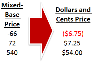
Data imports from other programs form the basis of a lot of the information we work with in Excel, and in the best of times, it arrives perfectly formatted and ready to be analyzed in the spreadsheet. Not every data import is equal, however, and occasionally, the numbers coming in don’t resemble anything that a human could read. Today, we have an inventory system from Mars which likes to store price information in a very non-standard way. In this poor computer’s mind, -66 means -$6.75, 72 means $7.25, and 540 means $54.00. In order to make sense of it, we’re going to have to break down the rules of this alternate notation and convert it into something we (and Excel) can use.

Examine the Data

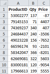
Before we can even begin to do a translation of units or bases, we need to look at our data set to make sure we understand how the notation works. Our example sheet has a column for ProductID, Qty, and Price.

The Price is what we need to focus on… Our translation rubric is as follows:

-66 means -$6.75

72 means $7.25

540 means $54.00

The right-most digit defines the cents after the decimal. The other digits and the sign define the dollars. The dollars are straightforward, but we need to understand how the cents behave.

6 means $0.75

2 means $0.25

0 means $0.00

It turns out that the numbering is consistent. We add $0.125 for each 1 added to the digit. Starting at 2 ($0.25), we add 4 to get 6. 4 * $0.125 = $0.50. Sure enough, $0.25 + $0.50 = $0.75.

This is great! It means we now have a rule for getting between Martian Inventory Pricing and plain old Dollars and Cents.

Breaking Down the Pricing Data

We need to separate the dollars part of the pricing data from the cents part, but there is a complication. We can’t just subtract the cents digit because it will change the negative price values. 66 – 6 = 60 ($6.00), but -66 – 6 = -72 (-$7.25) when we want -60 (-$6.00).

To make sure we always get the dollar value we want, we’re going to take the absolute value (always positive) version of the price. Excel does this with the ABS() function. The syntax is simple:

=ABS(number)

We’ll subtract the cents digit from the absolute value with the RIGHT() function, which has the following syntax:

=RIGHT(text, [num_chars])

We’ve used string parsing in other articles here and here if you want to see other examples…

The final formula to isolate the dollars value combines the two and divides by 10 to take away the zero at the end:

=(ABS(C2)-RIGHT(C2,1))/10

Thus, -87 becomes (87 – 7)/10 = 8.

Converting the Base-8 Digit to Cents

We have figured out the conversion rule for the Martian Cents Digit already (it’s essentially Base-8 instead of Base-10), so the math is simple. We’ll use the same RIGHT function as before:

=RIGHT(C2,1)*0.125

Thus, -87 becomes 7 * 0.125 = 0.875, which will round to 0.88 cents.

Stitching Together Dollars and Cents

The price is a number, so it’s easy enough to add the dollars and cents together:

=((ABS(C2)-RIGHT(C2,1))/10)+(RIGHT(C2,1)*0.125)

But this misses one piece. This formula would change -87 to 8.875. We need to restore the sign. For that, we can use this little arithmetic trick:

=C2/ABS(C2)

This will translate to 1 for positive numbers and -1 for negative numbers. Perfect! Multiply the dollars and cents by this value, and we’ll have the proper dollars and cents.

The final formula is as follows:

=(((ABS(C2)-RIGHT(C2,1))/10)+(RIGHT(C2,1)*0.125))*(C2/ABS(C2))

The formula can be dragged down to fill the rest of the cells in column D.

Converting Back to Martian Units

With a bit of formatting, we have successfully converted our Martian Inventory Prices to Dollars and Cents. But just in case we need to put prices back into the Martian Inventory System, we should figure out how to convert backwards.

Separating Dollars and Cents

We can approach the conversion the same way we did the first time, by separating the dollars and cents. It’s made a bit easier because we can look for the dollars with the INT() function. The syntax for INT is as follows:

=INT(number)

Put together, we can recover the dollars, strip the sign with ABS and multiply by 10 to return to the earlier format:

=INT(ABS(D2))*10

Converting Cents to the Base-8 Digit

Just like INT and ABS can pull the dollars from the value, the MOD() function and ABS can pull the decimal. The syntax for MOD is as follows:

=MOD(number, divisor)

By specifying the divisor as 1, MOD will calculate to the remainder, which will be the fraction after the decimal. We can then divide by 0.125 to arrive at the base-8 digit:

=MOD(ABS(D2),1)/0.125

Stitching Together the Martian Units

We’re close now… We can add together the converted dollars and the base-8 digit to get the full term:

=INT(ABS(D2))*10+MOD(ABS(D2),1)/0.125

But this still doesn’t have the sign restored, just as with the first conversion, and the same trick we used before will work. The final formula is as follows:

=(INT(ABS(D2))*10+MOD(ABS(D2),1)/0.125)*(D2/ABS(D2))

The formula can be dragged down to fill the rest of the cells in column E.

Mixed-Base Price Conversion Example

That’s it! Now your spreadsheet functions completely between the two units! You can look at the prices before they was converted on the first worksheet and after on the second spreadsheet. You can also download the sample file by clicking the Excel icon in the bottom right.