The Excel functions for performing ranking and establishing percentiles are poorly described and confusing to use on the best of days. The PERCENTILE function doesn’t give the percent ranking of the item, but the instead the value at a given percentile (which might not even exist!). This makes it difficult to calculate even simple percent rankings in Excel. But what if you want to rank a sub-set of a list based on some criteria? In this tutorial, we’ll walk through the challenges of calculating percentiles and ranking values based on filtering criteria using a basic example.

Examine the Data

For this exercise, we need a data set of values that can be filtered by a criteria. In this example, we’ll use a list of the populations of capital cities around the world. Our challenge will be to calculate the percentile ranking for capital cities within each continent separately. Let’s take a quick look at the data…

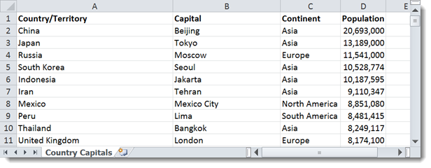
In this example, we can see that while it’s easy to see that Beijing has the largest population overall, it is difficult to see where other cities rank in population on each continent. They are all jumbled together!

There are two ways to approach this problem. If this data set is static and you will never need to update it, it may help to sort it by the criteria (in this case, Continent) and perform your rankings and percentiles from there. Let’s look at this option in detail.

Sort, Rank, and Calculate Percentiles using RANK and COUNT

To filter the data by criteria manually, we can perform a sort on it. Select the columns that contain the data. Then click the Sort button in the Sort & Filter section of the Data menu tab.

This will bring up the Sort dialog box. In the window that appears, choose the column that contains the criteria to sort by. In this example, it is the Continent column.

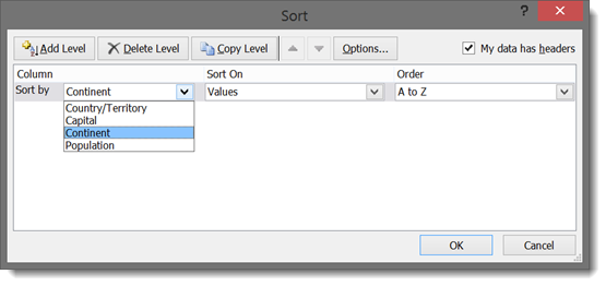
Click OK to apply the sort.

Now we can determine percentiles for each Continent separately. To do so, we will need to use the RANK and COUNT functions.

The RANK function gives the rank order of a value in a list. The syntax for RANK is as follows:

=RANK(number, ref, [order])

In Excel 2010 and newer, RANK has been re-named to RANK.EQ with the same syntax:

=RANK.EQ(number, ref, [order])

The number is the value you want to find the rank for.

The ref is the cell range that contains the list of numbers you want to compare it to.

By default, RANK and RANK.EQ will rank in descending order (largest number at the top, ranked 1st). The optional order can be a 0 for descending order (the default) or a 1 for ascending order (smallest number at the top, ranked 1st).

RANK will give us the “spot in line” for each value in our data, but to get a percentile, we need to know how many other values there are in the list. For this, we use COUNT. The syntax for the COUNT function is as follows:

=COUNT(value1, [value2], ...)

Each value in the COUNT function can be a cell or a range of cells. COUNT will count all the cells that have values in them.

Let’s find the percentile ranking of all the populations for African capital cities…

We want to compare the population of each row to all the populations in Africa to get the rank. Then we want to divide that rank by the total number of African cities there are in the list. The syntax for the formula in the first row is as follows:

=RANK.EQ(D2,$D$2:$D$58,1)/COUNT($D$2:$D$58)

D2 is the population in the first African city on the list.

The range D2:D58 is the list of all the African populations on the list. It has dollar signs ($) in front of the column letter and the row numbers to lock the range in place. We can copy the formula down the row for all African populations, and RANK will still compare each row only to the other African cities. COUNT will similarly only count the number of African cities in the list.

The RANK is put in the descending order (1) so that the largest population ranks 1st (100%) in the calculation.

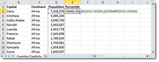
You can drag the formula in E2 down for all the rows that have African cities. After changing the formatting to show percentages, you will have the percentile ranking for each African capital city by population size!

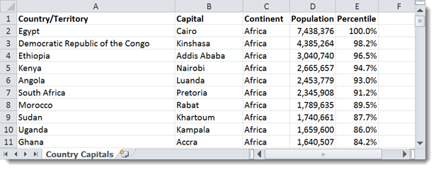
You can repeat the process for the other continents individually. You will have to manually change the ref range of the RANK function and the value range of the COUNT function to indicate the new continent set.

Automatic Conditional Ranking and Percentiles with SUMPRODUCT

The above process works for simple data sets and one-time sort and filter operations, but if you have a large data set or need to be able to refresh it and re-rank often, you need a more automatic way to do the filtering and sorting of criteria.

Fortunately, SUMPRODUCT can help us do just that using a trick called an array formula and Boolean (TRUE and FALSE) equations.

Boolean Equations in Excel

Excel can test equations to see whether they are TRUE or FALSE. For example, if you entered:

=1+2=3

Excel would show TRUE in the cell because 1+2 is equal to 3. Try an inaccurate comparison:

=1+2=4

Excel shows FALSE.

Pretty simple. The trick is that Excel can do  math with Boolean statements. It treats TRUE as 1 and FALSE as 0.

Try entering the following in a cell:

=TRUE+TRUE+TRUE

Excel will calculate the cell’s value as 3.

Using Boolean Arrays with SUMPRODUCT

SUMPRODUCT can use booleans an an array to filter results. If you compare an array to a criteria and  multiply it with itself, you’ll get a filtered sum, just like if you were using a SUMIF function. For example:

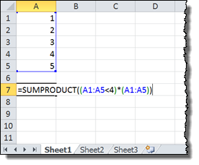
The above example evaluates to 6. It is comparing each row to 4. When the number is less than 4, it returns TRUE (or 1). When the number is not less than 4, it returns FALSE (or  0). The SUMPRODUCT multiplies that set of results against the same numbers and adds them up. 1, 2, and 3 are less than 4, so they are summed to get 6.

This is the same as if we did the multiplication and addition long-hand:

1 * 1 = 1
1 * 2 = 2
1 * 3 = 3
0 * 4 = 0
0 * 5 = 0
---------
        6 = (1 + 2 + 3 + 0 + 0)

Building a SUMPRODUCT Percentile Formula

We are going to apply the same strategy to filter the city populations by matching their continents in our example data set. We don’t even need to sort it first! Let’s go back to that original, un-sorted city list:

In the first row, enter the following formula:

=SUMPRODUCT(($C$2:$C$245=C2)*(D2>=$D$2:$D$245))/COUNTIF($C$2:$C$245,C2)

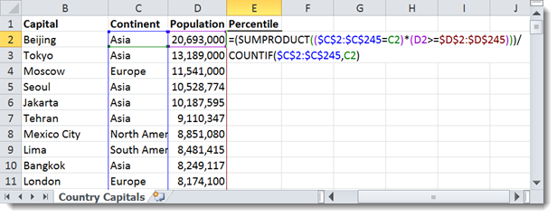
Pay attention to the locked ranges. They are selecting the entire column of data for Continent ($C$2:$C$245) and Population ($D$2:$D$245). Let’s examine what the formula is doing by looking at each of the Boolean statements:

($C$2:$C$245=C2)

This is comparing each row’s Continent to the continent in the current row. It will return TRUE for each match and FALSE for each mis-match. This means we will only be considering populations in the same continent.

(D2>=$D$2:$D$245)

This is comparing each row’s Population to the population in the current row. It will return TRUE for each value that is smaller than or equal to the current row and FALSE for each value that is greater than the current row. Remember, this will only count for populations in the same continent because of the earlier Boolean statement.

This is doing a conditional ranking, similar to the RANK statement in the manual example earlier in the tutorial. It’s just doing it for the un-sorted list. You could add or remove rows from the list and it would automatically re-calculate the rank.

The COUNTIF function is the same as the COUNT function in the manual, sorted example. It’s just counting only the rows that meet the criteria. The syntax for COUNTIF is as follows:

=COUNTIF(range, criteria)

In this case, the range is the continent column, and the criteria is the current row’s continent.

Now that the formula has been built, we can simply drag it down to all the rows in the data set. It will automatically calculate a separate percentile ranking for each country within its own continent!

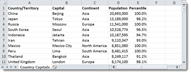
Note that the largest city in Europe (Moscow) is ranked in the 100th percentile for Europe even though it is third largest overall. This shows that the formula is working correctly!

Download the Example File

You can experiment with the example data in the embed below, or download the spreadsheet by clicking the green Excel button in the bottom right.