Quick Navigation
Cleaning Up the Helper Columns and Finalizing the List
Now we have everything we need to make our final comma-separated list, but first we need to clean up our helper columns.
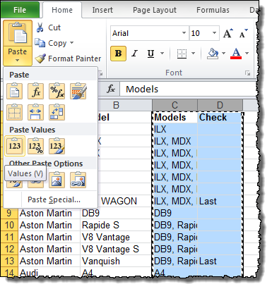
The Models and Check columns are currently dependent upon the order of the rows, so we need to lock the formula output with a Paste Values command. Paste Values replaces the formulas in each cell with the current output of the formulas.
To do so, select columns C and D and press CTRL+C to copy the cell contents.
Then click the Paste button from the Home menu tab and choose Paste Values as shown below:

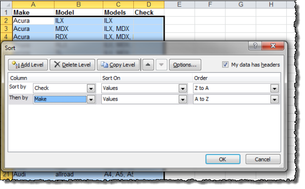
Now we can safely re-sort our data to identify the complete lists. Select all of the columns from A to D and choose Sort from the Data menu tab.

Choose to sort first by the Check column (sorting in Z to A order to bring the Last values to the top), and then by Make using the normal sort direction. When we click OK, the rows marked “Last” will rise to the top.
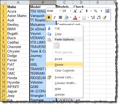
Now, we can safely delete the Model column, leaving only the Models. Select column B, right-click the selection, and click Delete from the menu.

We can also eliminate all the partial lists that aren’t marked as “Last”. Select rows 44 (in our example data set) to the end of the worksheet, right click the selection and click Delete from the menu.
What we are left with is a single row of comma-separated Models for each Make of vehicle!
Bang on !!! Super trick..Thanks…
This helped article me so much! Thank-you for creating this site. Now that I’ve found it I know that I will be visiting quite often. — Janine
Thanks and it helped.
You have no idea how much time this just saved me. Hours upon hours as we calculate the duplicate registration for our client’s conference attendees.
Tricks like these help us clean up our data and provide the clearest picture for our clients. A HUGE thank you!
Thanks so much for sharing this. I was doing this manually for a list of streets and page numbers for a mapbook and this saved me loads of time. Great tutorial!
Thanks Andrew for your Clear article , saved me a lot of time with a huge excel file.
THanks a lot!!! you are super!!! Great logic used
simple and elegant solution; i found veryy very help…i hope to impress my boss ::
thanks!
Very clear and helpful. Thanks a lot!
This is a solution I’m keeping. Very clever.
Hi,
This is brilliant. I have 2 more layers of complexity in the Model column in the situation I am facing.
Here, there is only one model for one cell/row. In mine, for say Row 2 – Column A – ACURA, Column B Model is say – ILX, MDX, RLX,
There may also be repeat Models as well for eg, Row 3 – Column A – ACURA – Column B – Model is MDX, RLX,
So when I concatenate, I have the value for ACURA as ILX, MDX, RLX, MDX, RLX. – How do I clean that up to just show ILX, MDX, RLX?
Thanks! I need to send this in by 8 AM EST which I am sure would not be possible but any help would be extremely appreciated!
– Harish
Hi Harish!
A couple years late for your deadline, but in case this helps other people, this is what I recommend:
Before you use this tutorial to concatenate your data into a comma-separated list, you need to break out your data into individual items. You’re basically going to have to reverse this concatenation process until you get your list down to:
Acura ILX
Acura MDX
Acura RLX
Acura MDX
Acura RLX
Other tutorials on the internet may help you with this problem, but I suggest starting with the Text-To-Columns feature of the Data tab in Excel.
Then, you can use the “Remove Duplicates” feature of the Data tab in Excel to eliminate the extra MDX and RLX lines in your data.
Finally, you can use this tutorial to get the non-duplicated list to group up again.
Good luck!
Andrew
Thank you! Saved me hours of trouble 🙂
Thanks for the great time saving idea saved lot of hours
Awesome. I couldn’t get my head around this but your method makes so much sense. Thank you!
Thank you very much for this tip!! Really useful.
Thanks so much! This was exactly what I needed and the example made it very easy to understand!
Thanks for the clever trick.
Thank you SO MUCH! You totally rock!
Thank you a ton!!!
OMG!! You are a lifesaver! I have worked all day manually merging values on a 13,000 row spreadsheet!!!!!!!!!!!!!!!!!!!!!! This literally took it down to under 1,200 in about 5 minutes. Thank you thank you thank you!
Woowwwwww… thanx alot Andrew Roberts..
I was dying to know this “absolute brilliant formula” and u made it extremly easy.. thanx again
You save my life..
Hey great tutorial. Worked for me. Thanks a lot.
This is great! One follow up questions… What if you wanted to show an as of date either before or after the selection? I can’t keep it from wanting to repeat the date. Any solutions?
Dude! You da real MVP! Company has been doing this manually for ages. Made me look like everyone’s Saviour.
IS THERE A WAY TO APPLY A CONDITION THAT IF THERE IS NO VALUE IN THE ASSIGN CELLS DO NOTHING (=IF(K111=K110,O110&”, “&M111,””)???
this handles empty cells:
=IF(AND(B2=B1,D1″”,D2″”),E1&”, “&D2,””&D2)
If you just want to transpose a single column into a comma separated list, I find this utility helpful:
http://convert.town/column-to-comma-separated-list
Thanks, that is useful. Quicker than writing the formula to do it.
Thanks this is great. I have been trying to find a way to do this for ages.
I am cuurently trying to concate several dates and I can’t get the first date to format correctly. Subsequent dates do format.
I’m using =IF(A46=A45,BB45&”; “&TEXT(Y46,”dd/mm/yy”),Y46)
which gives me 41761; 29/04/14; 28/02/14
Any help would be much appreciated.
Thanks a lot…this trick was really helpful and saved a lot of time
This is great! How can I do this when I have multiple columns of data? For example, what if this example also had columns for color, year, and transmission?
Hi, Great article! It’s exactly what I’m looking for; however, do you have a quick tutorial on how to do the process backwards?
I was given a row with multiple model #’s, however want to split it up into individual rows. How can i go about this?
Thanks again!
You might look to the Text-to-Columns feature in the Data Tools section of the Data menu tab. This should let you break out the models into individual cells. Good luck!
This trick was very helpful and helped save time!
I added this formula to a massive file. Now, how do I delete all of the records that I don’t need any longer without manually doing it one by one?
Sounds like you need to build the “check” helper column still… Look at page 3 onward: https://www.exceltactics.com/combine-data-multiple-rows-one-cell/3/
Thank you~!!Saved my bacon with this 🙂
I’ve been wasting many hours to merge my data. your solution is so cool. you save my day.
Hi.
How would i reverse this process. I get my data the other way around and need to sort it like the first page. Thanks in advance
Thanks for your sample formula. Really help me to collect data.. 🙂
Thanks a lot,
Francesco
Excellent.
I was using the concatenate function differently that was consuming me more time.
Thanks so much for the information.
Regards,
Edward…
THANKS SIR JI
Thanks. this saved me a an hour. I needed to create a list of 150 sales reps and the states they cover. Added an additional if to compare the states and voila, a useful list.
THANKS SIR JI
This is just beaaautiful!! Thank you so much!… Wonderfully explained.!
Lifesaver. Thanks for this!
Thank you!
so nice and simple post and resolved the issue
Thanks a lot
Awesome Bro, Its great logic, works perfectly…
Thanks ! worked for me 🙂
Thanks Sir, very helpful video…
Thank you!!
I have used it successfully. In addition to this, i have to extract first (left) 5 characters from the concatenated cell and put it in another cell.
thanks
This is awesome! Is there a formula for the reverse process? I have a list with values in one cell separated by commas and I need to convert it to each value is in a separate row.
Well good, thank you!
This was a GREAT video. It helped ALOT when we were combining 10,000 lines. I knew the combination needed an If function but could not develop the formula.
Awesome Bro, Good logic, Thanks Lot.
Good stuff. This helped me 🙂
What I was searching for days..!! Superb guide. Many thanks..:)
This is great!
I had to combine students attendance and academic standings in order to use V-look up successfully. It’s always great to find helpful and clear tips for Excel. Thank you!!
Helped me for large data consolidation, thank you very much !!
Thank you so much! You don’t understand how much this helped me!
Thank you. I have used it for our Civic Association for a membership reminder. There are a few tables in the dbase (place,member,payment,owner etc) and more than one member with an email address for the same properties. This helped me to use only unique email addresses to send personalized letters to members with a list of ALL the properties included and not a email for every property. I did find a small program from a third party, but will have to pay more than R500 to use it 4 times a year.
I HAVE THE DATA IN DIFFERENT COLUMNS LIKE A, B,C, D E, F, G etc but all the cells are not filled, I want that the data in different columns must be copied in a single column say for example H. How ??
Hello,
I’m using excel 2010. When I use your method, all rows except the last return 0. The last returns the first value. Any suggestions?
Thanks,
JJ
Yay!
Every other solution I found required purchasing an add-in or creating a macro.
Thank you <3
This is genius, thanks!!
Thanks so much for this. Almost every other site provided really complex VBA code based solutions. This on the other hand was a really simple and elegant solution. Thanks again!
You are the best !!! Saved a lot of my time 🙂
thanks a lot man, much appreciate , works flawlessly
Brilliant and very helpful post. was thinking of doing this by taking to sql server then realized there could be soln in excel. This one helped a lot. Thank You so much..
Excellent trick dude, but I have one question is there any data row limit in this formula. When i Tried using this in my data set it stuck 2043 rows. Please help.
Well played sir. Very much appreciated. You even expanded my knowledge of different ways to achieve concatenates 🙂
Fantastic!!
Thanks a ton & I can’t thank you enough.
Thanks this article really help me
Thank you so much! This really helped me with my data analysis.
Well done Thanks a lot !!!
Thanks so much for this tutorial!
This helped me consolidate thousands of lines of data for a vendor’s template without me going crazy or needing to pester coworkers over the holidays.
You rock!!
Oh man, this saved me a couple of hours work! Thanks for sharing and keep it up!
This was an AMAZING video!! I greatly appreciate this tutorial. I learned so much. THANK YOU!!!
You’re great man! Wish you good day and much more trainings 🙂
It helped a lot.
Thank you so much for this trick! Saved by from concatenating hundreds of values manually!