With the combination of INDEX and MATCH functions and Excel’s powerful array formulas (entered using CTRL+SHIFT+ENTER), we can already make Excel do the hard work of looking up data with multiple criteria for us. I wrote about it in the article How to VLOOKUP with Multiple Criteria Using INDEX and MATCH, and you should definitely check it out first if you need to use multiple conditions when looking up data in Excel.

The only downside of the INDEX/MATCH method is that it takes a lot of crunching to get its results. If you just need to look through a couple hundred, it does a great job! If you’re working with truly big data sets numbering in the thousands or hundreds of thousands of rows, you might need something that can work faster… This tutorial will show you how to combine CONCATENATE and a helper column to make VLOOKUP faster than ever!

The formula INDEX/MATCH from the VLOOKUP with Multiple Criteria article is computationally intensive because it uses an array formula to compare all the values in both criteria columns to find what you are looking for. If you have thousands of rows, this means it has to check them all twice for every single lookup. If you put this array formula in multiple tables, you are doing the work of looking up the matches many, many times, and this can slow your computer to a crawl, make you run out of memory, or even crash Excel!

Making a Helper Column

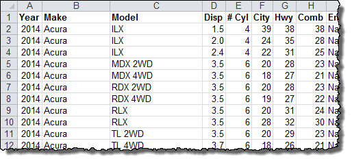
The secret to speeding up the multiple criteria lookup is to split up the task of combining the criteria and doing the lookup. To do this, we need to add a column to the data set and combine the criteria we want to lookup. Let’s use the same example data set as the last tutorial:

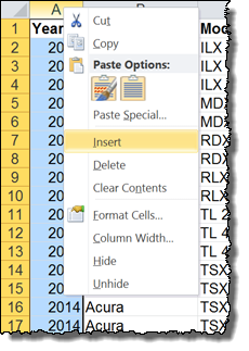
Let’s try to recreate the same lookup as before. We want to be able to look up the Model (Column C) and the Displacement (Column D) of the car we want to be able to find out the Combined MPG (Column H). To do this, we need to insert a helper column that is there just for us to look up against. Right-click Column A and click Insert to add a column at the beginning of the sheet.

We are going to use CONCATENATE to combine the Model and Displacement information for each row in one column. The formula for the first row (in A2) is as follows:

=CONCATENATE(D2,E2)

You can drag the formula down the entire column, or copy and paste it down the sheet. The final result should look like this:

You can see that having both columns together in one makes each row have a unique identifier. “ILX1.5” is different than “ILX2.4” even though the Year, Make, and Model aren’t different for those rows. You can do this for any number of columns, which means you could use it for 2, 3, or 10 criteria and it wouldn’t require any extra computational work!