The business world is full of forms and paperwork built out of Excel spreadsheets. Even though the program isn’t designed for the task, the benefit of being able to calculate sums, totals, etc. in the form makes it the de facto standard for invoices, receipts, shipping manifests, and purchase orders everywhere. Often, you’ll find yourself using the same forms over and over again, so it makes sense to automate as much of the process of filling them out as possible. I’ll show you how to automatically fill addresses and contact information into a template shipping manifest…

Examining the Form and Data

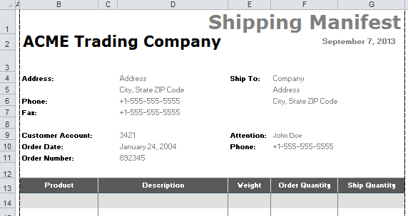
First, let’s look at our existing form. It has standard fields for Company Name, Address, City, State, ZIP Code, Phone Number, and Contact Name. All of them have to be manually entered right now.

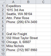
Then, let’s examine the data. The information we need is all there, but it is saved in plain list, which makes it very difficult to search through, sort, and find things in.

Cleaning Up (Scrubbing) the Address Data

In order to work with the address data, we need to re-format it into more predictable columns and rows. Ideally, each entry should have it’s own row, with a column devoted to each data point. Since there is a manageable number of entries in our example, it is probably easiest to manually repair the data set. Were this a longer list, it may be worth crafting a formula or two to pull out the information. The result of our data scrubbing looks like this:

Creating a Drop-Down List Box

Now the the data is cleaned up and organized, we can start to work with it in Excel. First, we are going to create a drop-down box under the Company Name field in the Shipping Manifest. This will make it easy to choose which shipping information we need. When new shippers are added, they can be added to the new data table and they will automatically be added to the list.

Select the data entry cell for Company next to Ship to:

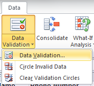
Under the Data menu tab, choose Data Validation and then click on Data Validation.

In the Data Validation dialog box that appears, under Allow section, choose List. Then click the data field next to Source.

Switch to the Shipping Addresses tab and select column A. Then click OK.

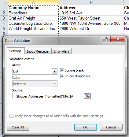
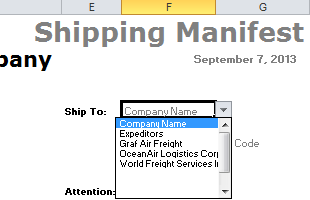
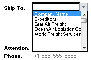
If you go back to the Manifest sheet, you can look at the Ship to: data field and find the drop down box. It will show you your available options.

Automatically Filling the Data Fields

With the drop down box complete, we need to start linking the data fields to the output. Select the data entry cell for Address under the company name (F5 in the example).

To find the correct address information, we’re going to use an Excel function called VLOOKUP(). The syntax for VLOOKUP is as follows:

=VLOOKUP(lookup_value, table_array, col_index_num, [range_lookup])

The lookup_value is what we’re looking for in the table. In this case, that’s the company name, which is in cell F4.

The table_array is the set of rows and columns that we want VLOOKUP to scan for a match. The first column must have the lookup_value in it. In our case, the value is the columns of the Shipper Address tab.

The col_index_num is the column of the table_array we actually want to appear in the cell. In this case, it is the address column, which is the second column (column B) of our table_array.

Finally, range_lookup tells VLOOKUP whether we are okay with close matches instead of exact. We need an exact match, so the value will be FALSE.

If VLOOKUP doesn’t find a match in the table, it throws an error, which isn’t good if we need to enter an address that isn’t on the Shipper Address list. To handle the error and keep the form clean, we’ll wrap the VLOOKUP in another function called IFERROR(). The syntax for IFERROR is as follows:

=IFERROR(value, value_if_error)

The value will be the VLOOKUP function.

The value_if_error will just be an empty string (“”) so the form stays blank when there is no company selected.

The final formula for the Address field is as follows:

=IFERROR(VLOOKUP($F$4,'Shipper Addresses (Formatted)'!A:G,2,FALSE),"")

The process will repeat for Contact Name and Phone Number. The same formula can be used, but the col_index_num will change accordingly.

The formula for Contact Name will be in cell F9 and is as follows:

=IFERROR(VLOOKUP($F$4,'Shipper Addresses (Formatted)'!A:G,6,FALSE),"")

The formula for Phone Number will be in cell F9 and is as follows:

=IFERROR(VLOOKUP($F$4,'Shipper Addresses (Formatted)'!A:G,7,FALSE),"")

Automatically Filling City, State, and Zip Code

The City, State, and ZIP Code data are held in separate cells, so we’ll need to stitch them together using multiple VLOOKUP functions. Otherwise, the process is the same. To stitch them together, we can use the CONCATENATE() function, which turns multiple strings into one long string. The syntax for CONCATENATE is as follows:

=CONCATENATE(text1, [text2], ...)

For example, =CONCATENATE(“to”,”get”,”her”) calculates to “together”.

The formula for City is as follows:

=IFERROR(VLOOKUP($F$4,'Shipper Addresses (Formatted)'!A:G,3,FALSE),"")

The formula for State is as follows:

=IFERROR(VLOOKUP($F$4,'Shipper Addresses (Formatted)'!A:G,4,FALSE),"")

The formula for ZIP Code is as follows:

=IFERROR(VLOOKUP($F$4,'Shipper Addresses (Formatted)'!A:G,5,FALSE),"")

We’ll need to stitch them together with CONCATENATE and add the proper commas and spaces. The final formula for the City, State ZIP data field is in cell F6 and reads as follows (on one line):

=CONCATENATE(IFERROR(VLOOKUP($F$4,'Shipper Addresses (Formatted)'!A:G,
3,FALSE),""),", ",IFERROR(VLOOKUP($F$4,'Shipper Addresses (Formatted)'!A:G,
4,FALSE),"")," ",IFERROR(VLOOKUP($F$4,
'Shipper Addresses (Formatted)'!A:G,5,FALSE),""))

Automatically Filled Shipping Manifest Example

That’s it! Your drop-down box now automatically fills in the Address, Contact Name, and Phone Number on the Manifest! You can play around with the example before it was scrubbed and automated on the first two worksheets and after on the second two spreadsheets. You can also download the sample file by clicking the Excel icon in the bottom right.