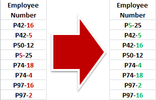Excel’s built-in sort functions are incredibly useful for organizing data and ordering information like dates, times, and other numerical inputs. Sometimes, though, you may need to sort product IDs, employee numbers, or other information that has letters and numbers in it. Then, what do you do? A normal Excel alphabetical sort will not prioritize the numeric parts of a string on its own. Here is how to sort alphanumeric data with complete control…

 

Looking at the Data

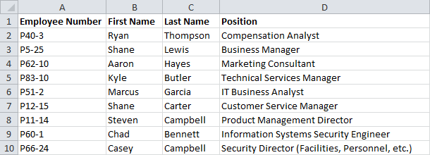
Let’s imagine you have a list of employees. It might have their first name, last name, and job title. All of these are easy to organize around – they are all pure text. Adam comes before Bethany. Smith comes after Johnson. Accountant comes before Technician.

Maybe these employees have an employee number that is based on when they were hired or what division they were recruited from. This might have a different structure like “P<dept_number>-<recruit_date>”. It might make sense to sort the employees by department number first and then by recruit date… Let’s see if Excel is smart enough to do this on it’s own.

Trying a Normal Sort

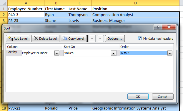
Select the columns of data you want to be affected by the sort. If you are following along with the example, it’s A:D. Then click on the Sort button on the Data tab of the menu.

Choose to sort by the Employee Number field and click OK.

Let’s see how well it worked. On first glance, it might look like it did the trick… The first numbers after the “P” are sorted, but wait…

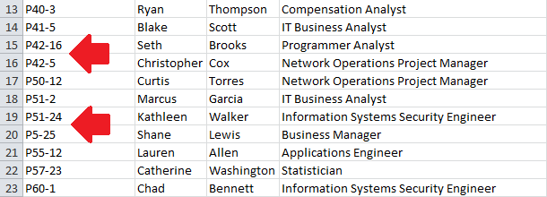
For some reason, Excel thinks that “P51” comes before “P5”. And “P42-16” is sorted in front of “P42-5”. How is this possible?

Since the cells contain text as well as numbers, Excel treats the entire cell like a text string. It sorts according to the order the “letters” appear instead of the entire number (e.g. the “1” in “P42-16” comes before the “5” in “P42-5”).

We’re going to need to do a bit more work to make Excel do our bidding…

Creating Sort Columns

To get around Excel’s annoying handling of numbers in text, we’re going to create a couple of columns to sort with. They’ll keep the original cell un-changed, but let us re-arrange the data how we’d like.

Select the column to the right of the mixed cell you want to sort (Employee Number in this example). Right-click the column labels and click Insert to add a column.

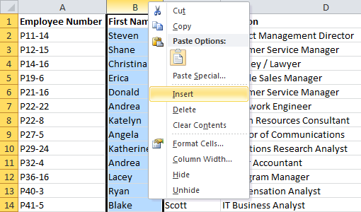
Press CTRL-Y to repeat the action and add another column.

Finding the Sort Data

We are going to use a combination of functions that look at text data to pull the numbers out of the mixed string (another article uses similar string parsing tactics to change notation). First, we’ll tackle the number after the “P” in the example, using the MID() function. The syntax for MID is as follows:

=MID(text, start_num, num_chars)

The MID function can take part of a string, but we need to tell it where to start and finish. Some of the numbers are single-digit and others are double-digit, so it’s not as easy as looking for the second character. We need to focus on what makes the numbers similar. In this case, they all come after the “P” and end right before a “-” (hyphen).

The start character in this case is always the second (after the “P”), so we can specify it directly, so start_num is 2.

The number of characters in the first number is different each time, so we need to be more sneaky. We’re going to count the number of characters before the hyphen using the FIND() function. The syntax for FIND is as follows:

=FIND(find_text, within_text, [start_num])

In this case, we’re looking for the hyphen, so find_text is “-“. We don’t need start_num this time.

The FIND function is going to report the location of the hyphen in the Employee Number, but we need to tell MID how many characters to pull from the string, so we’ll have to subtract 2 from the FIND result: 1 to get in front of the hyphen and 1 to discount the “P” at the beginning.

The MID function is going to provide the part of the Employee Number that we want, but it’s still going to be text. When we sort, we need it to be a number, or the sort will treat it the same as it did in the first attempt. For that, we wrap it in a VALUE() function. The syntax for VALUE is simple:

=VALUE(text)

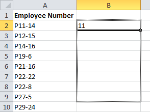
The final formula for the first sort cell (B2 in the example) is as follows:

=VALUE(MID(A2,2,FIND(“-“,A2)-2))

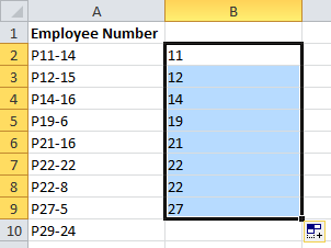
The formula is complicated, so rather than type it again, you can drag it down and Excel will automatically change the cells as necessary:

 

Sorting After the Separator

Now we need to extract the number after the hyphen in the Employee Number. We’re going to use a similar strategy, but we need a couple additional formulas. We could use the MID function, but it would be cumbersome since the cells are different lengths. Instead, the RIGHT() function will pull characters from the end of a string. The syntax for the RIGHT function is as follows:

=RIGHT(text, [num_chars])

The RIGHT function needs to know how many characters we need, so a FIND function isn’t enough. We also need to know the entire length of the string to find out how many characters are after the hyphen. For that, we’ll use the LEN function. The syntax for the LEN function is easy:

=LEN(text)

If we subtract the location of the hyphen from the total length of the Employee Number, we’ll have the exact number of characters needed for the RIGHT function. Finally, we wrap the entire formula in another VALUE function to make sure we get the number instead of the text.

The final formula for the second sort cell (C2 in the example) is as follows:

=VALUE(RIGHT(A2,LEN(A2)-FIND("-",A2)))

When you’re sure it works, drag down the formula to fill in the rest of the cells. To make them easier to find, you can title the columns – I called them “EN Sort 1” and “EN Sort 2“.

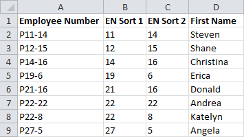
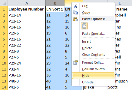
Now that the columns are created, we can safely hide them from view, since they aren’t important to reading the data. Just select the two new sort columns, right click the header, and click “Hide” from the menu.

Sorting with the New Sort Columns

Select the new sort columns (B:C). Then click on the Sort button on the Data tab of the menu.

Choose to sort by the EN Sort 1 column. Click the “Add Level” button to specify a second sort criteria. Choose to sort by the EN Sort 2 column in the second level. Then, click OK.

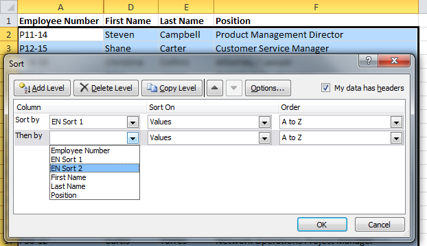
Examine your data. See how nicely it behaves? Good work!

Alphanumeric Sort Example

Below is the workbook example from the tutorial. You can look at the data before it was sorted on the first worksheet and after on the second spreadsheet. You can also download the sample file by clicking the Excel icon in the bottom right.