We often use Pivot Tables in Excel to make large data sets easier to read. Pivots let us organize huge flat files by putting dates or categories into their own columns, making them easier to read.

Sometimes, though, we need the exact opposite format for our data. If you receive data that is already pivoted and need it converted from columns back into individual rows, you’ll need to unpivot the table to get your results. Fortunately, Microsoft has a very powerful free plug-in for Excel called Power Query that makes this very easy to do! This is a tutorial to walk through how to unpivot existing data using Power Query.

Examine the Data

Here, we have a sample data set. It’s just a basic collection of sales volumes for different regions, broken down by month. Typically, this is how we like the data to look, but if we want to manipulate it in a Pivot Table of our own, we need to un-pivot it. To do so, we need to activate or install the Power Query plug-in for Excel.

Installing Power Query for Excel

Some versions of Excel (2013 and newer) have Power Query already built in. Others, including Excel 2010 and 2007, need it installed. Regardless of the version of Excel you have, running the Power Query installer will activate Power Query for you.

Click here to go to the Microsoft Download Page for Power Query

 

Click Download…

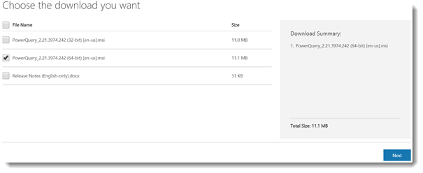
A pop-up will ask you to choose the version of Power Query you need – either 32-bit or 64-bit. You should choose the version that matches the version of Excel you have installed. If you aren’t sure which one to choose, try the 32-bit version. If that doesn’t work, you may need to download the 64-bit version instead.

Click Next, and the installer should automatically download. Run the installer program to install Power Query. You will know you have done it correctly when you re-start Excel and can see the Power Query tab on the toolbar ribbon.