Quick Navigation
Loading Data into Power Query
Open up your data set in Excel. Make sure you can see the Power Query tab on the ribbon toolbar. If you can’t see it, you may need to restart your computer or re-install Power Query because Excel cannot see the plug-in.
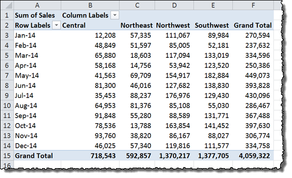
Select the cells that hold your pivoted data.

Select the Power Query tab on the ribbon toolbar and choose the From Table button under the Excel Data section.

A dialog box will pop up asking you to confirm the range where your pivoted data exists. Make sure you’ve selected the row with the column titles in your data and that the My table has headers option is checked.
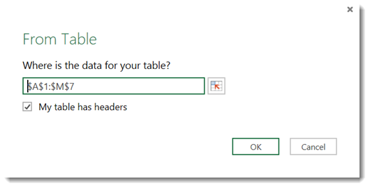
Click OK.
Power Query will automatically turn your pivoted data into an Excel data table and launch a Query Editor window.

Unpivot the Data in Power Query
Select the columns you wish to unpivot. You can either hold CTRL while clicking them individually or click the left-most column, hold SHIFT and click the right-most column.

Right-click one of the column headings you’ve selected to pull up an options menu. Click the Unpivot columns… menu item near the bottom.
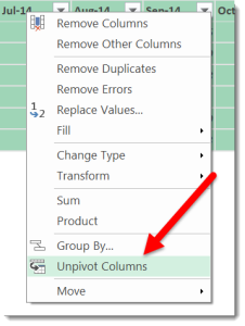
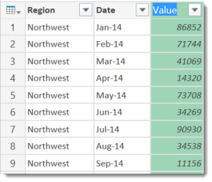
The columns will converted into their own unique rows in the data inside the Power Query window. By default, the pivoted column headers will be in a column called Attribute and the data in the table will be in a column called Values. You can change the new column names by double-clicking them and typing in your new header names.
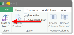
When you are satisfied with the new unpivoted columns of data in the Power Query window, click the Close & Load button in the top left of the toolbar. This will load the newly un-pivoted data back into Excel.
Review the Results of Unpivoting the Data
The new table will be inserted into its own tab in the original Excel spreadsheet.
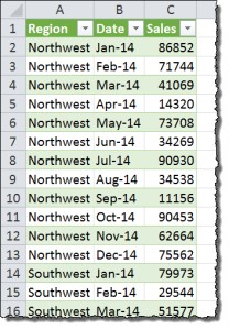
You can now use your freshly unpivoted data to combine it with other data sets, import it into a database, or build your own pivot tables!
That’s a great technique. Another solution is to use some of the tools and plugins that have solved this classic issue with dedicated buttons. For instance this one here: https://www.powerusersoftwares.com/unpivot-table lets you select a table and it will be flattened on another excel sheet
I have some medical data for staff including costs. I need to arrange it so that each hospital shows its totals in the first table and each patient total cost is also shown in a second table irregardless of whichever hospital they visited. Please help
Thank you so much for this article! This is so cool and helpful. I had been looking for this kind of technique for long time and I finally found it.