One of the most powerful features of Excel formulas is the ability to create absolute references that don’t move around when you drag to extend cell formulas or copy them to different places in your spreadsheet. Most Excel users figure out how to lock these references by either toggling through the options with the F4 key or using the $ (dollar sign) symbol in front of the column and/or row references.

When you start using data tables in Excel, many users are frustrated to discover that the normal methods for freezing the row or column references don’t work! This can make it time consuming to build your spreadsheets when they use tables. Fortunately, there are some workarounds! We’ll walk through a few of them in this quick tutorial…

Why Do We Use Data Tables in the First Place?

If you are wondering why you’d even want to use data tables instead of just nicely ordered cells in Excel, it’s probably worth a quick refresher…

Data tables in Excel are useful specifically because they grow and change to accept new data when it is added to the table, without needing to update formulas or references. This is hugely valuable when you want to copy and paste data into a spreadsheet from an external source to keep it up-to-date. In a data table, you can create calculated columns that reference other parts of the data table. When new data is added, the calculated columns will automatically update with the new information and new rows!

Summary formulas like SUMIF(), COUNTIF(), MAX(), MIN(), and AVERAGE() can be designed to reference the entire table or specific columns, and then automatically change to update their ranges when the tables grow or shrink!

The flexibility of data tables makes them the first choice for working with structured information, so that just means we need to learn how to work with them! Keep reading to find out how!

How Normal Data Table References Work

Data Table Column References

When you are working with data tables in Excel, the cell references look a bit different than the usual A1 letter-number combination for column-rows. This is because each row of the table acts like it is in its own 1-row spreadsheet. That means that the references only need to refer to the table name and the column. The row is assumed to be itself.

Let’s look at a simple table:
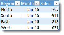If we wanted to add up all of the Sales column in the data table, the formula would look like this:

=SUM(Table1[Sales])

Output for this formula would be:

3167

Notice that it doesn’t ask for starting or ending row. It just asks for the column and table name.

Now, let’s add data to the table:
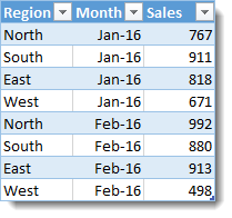The formula for summing the Sales column stays the same:

=SUM(Table1[Sales])

Now, though, the output for this formula has updated automatically:

6450

Without doing anything, the calculations accommodate extra data! No need to change references in the SUM() formula!

Data Table Example With Multiple References

Let’s show one more formula example using the same table:
Instead of creating a formula outside the table, let’s add a calculated column to add up the total for each Region. Name a new column to the right called Region Total. In the first cell of the column, enter the following formula:

=SUMIFS([Sales],[Region],[@Region])

It should look like this:

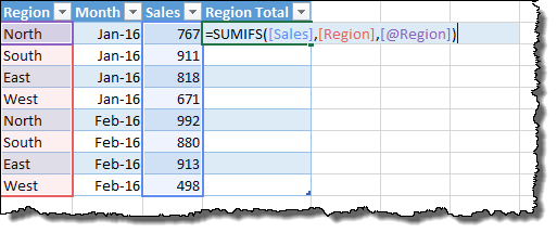
Note that the final term – the criteria for the SUMIFS() – uses the @ (“at” symbol). This notation means you are referring to the value of the Region column in the current row. Just press ENTER to populate that formula in the entire column, and you can see the result of this reference in the completed table.

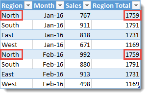
The SUMIF() calculation sums all the Sales for each Region, giving a matching total for every row from the North region (and for each of the others as well).

Now that you can see how powerful Excel data tables can be, you’ll probably want to use them… To build complex formulas quickly and reliably using data tables, you need to be able to lock references, so that’s what we’ll learn next… Click onward!

How to Build Locking References

Normally, it’s easy to build out columns and rows by locking references in formulas using F4 or adding dollar signs to the row and column of the reference… This lets you drag formulas down multiple rows or across multiple columns to quickly build a working spreadsheet.

Example of Normal Relative and Absolute (Locked) Cell References

Take this simple example:

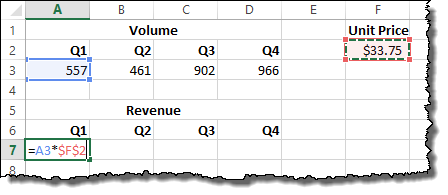
Here, we build a formula to calculate quarterly revenue based on volume and unit price. The volume will change each quarter in the new column, but the unit price will stay the same, so we lock the reference by pressing F4 or typing the dollar signs for $F$2 manually.

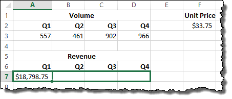
Once the formula is entered, we click in the lower right corner to drag it across the columns for the other quarters.

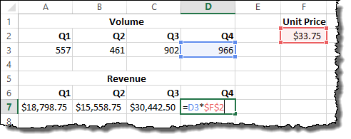
When we release the click, the formulas for each quarter are calculated. The cell reference for the volume cell (in blue) stays a “relative” reference that moves with the location of the formula cell. The reference for the unit price (in red), however, has become “absolute”, meaning it is locked to it’s original location.

Creating Absolute (Locking) References in Data Tables

Unfortunately, using F4 or adding dollar signs doesn’t lock references in data tables. It doesn’t even calculate the cell, instead throwing an error. Fortunately, there is a way to achieve the same behavior, but it requires using Excel’s data table syntax we spoke about above.

The easiest way to show how this is done is to walk through an example. Let’s combine the two sample data structures we’ve been working with to design a problem to solve in the next section. Click Next to continue!

How to Build Locking References in Data Tables

Sample Data

Let’s expand our Regional Sales table to a full 6 month period. This might be how your data could look if you were importing it from a database or other reporting software. It’s very machine-readable but not very human-readable. In this example, we are going to name the table in Excel as DataTable.

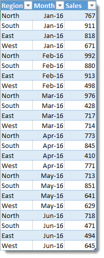
Now, let’s build a table to pivot the data into a more readable format. In this case, our goal is to have a separate column for each month and a separate row for each region:

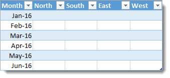
This table will be called PivotTable. To fill this table with data, we are going to use another simple SUMIFS() formula, but we will be working inside a table and looking up information inside another table…

Building a Formula that Refers to Locked Data Table Columns and Rows

Starting in the North column and the Jan-16 row, build this formula:

=SUMIFS(DataTable[[Sales]:[Sales]],DataTable[[Region]:[Region]],B$1,DataTable[[Month]:[Month]],PivotTable[@[Month]:[Month]])

It will look like this:

We’re locking references in three separate ways in this formula:

1. Referring to an entire locked column in a data table.
2. Referring to the current row of a locked column in a data table.
3. Referring to the locked header row of a data table.

Each of these uses slightly different syntax, so I’ll show each of them in order:

1. Locking Entire Data Table Columns

Normal data table column references look like this when you are inside the same table:

[Sales]

When you are outside the table the column resides in, they look like this:

DataTable[Sales]

The trick to locking the reference for the column involves treating it like a range of columns that only includes itself. You must also always reference the table name, even from within the table. Thus, the locked data table column syntax looks like this:

DataTable[[Sales]:[Sales]]

2. Referencing the Current Row of a Locked Data Table Column

Normal current row references for data tables look like this when you are inside the same table:

[@Month]

When you are outside the table the column resides in, they look like this:

PivotTable[@Month]

Similar to locking the entire column, as seen above, the trick to locking the current row reference is to treat it like a range, but the @ symbol is only used in the beginning of the range reference:

PivotTable[@[Month]:[Month]]

3. Locking a Data Table Header Reference

Working with Excel data table headers is a bit difficult because Excel treats them like fixed elements. That means it won’t remember that they are dates or other special types of data. They become field names. The assumption is that the number of columns in your data table won’t change over time – just the number of rows.

This means that to reference a header in a data table in a formula (and let that formula stay drag-able), you need to lock the reference. Fortunately, the header row of a data table always stays in the same place, so you can lock it like a normal cell reference in Excel. In the example formula above, that’s exactly what we did:

B$1

This notation ensures that when the formula is dragged across, it will reference Row 1 in the current column at all times. (The row number is locked, but the column is still relative.)

Completed Data Table Formula

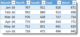
After dragging the formula down and across your new PivotTable data table, you should see the equation change dynamically to populate the rest of the cells.

The new formula in cell E7 reads:

=SUMIFS(DataTable[[Sales]:[Sales]],DataTable[[Region]:[Region]],E$1,DataTable[[Month]:[Month]],PivotTable[@[Month]:[Month]])

Done correctly, the formula looks very much the same in each cell of the data table! The only thing that will change are references to the header row of the data table, since these are normal locking references for Excel cells.

This is the final data table, complete with pivoted information. It’s much easier to read, and can be used to build charts and other reporting outputs as necessary.

Get the Excel Add-In to Map “Locking Data Table References” to F4

This process of adding ranges to all your data table references to make them absolute might be a hassle if you need to do it often… Fortunately, Jon Acampora over at Excel Campus has built an add-in that will map these locking ranges to the keyboard as F4 so they work just like normal absolute references in Excel.

You can check out his add-in here: Absolute Structured References in Excel Table Formulas