Using SUBTOTAL to SUM a Filtered Table

Let’s try replacing SUM with SUBTOTAL in the Total row of the table. First, we should remove the filter on Region so we can work with the entire table at once. Click on the filter icon by the Region header, choose the Select All option in the drop-down menu, and click OK.

The SUBTOTAL function in Excel works as a kind of master function for many others. It can perform the same function as AVERAGE, COUNT, COUNTA, MAX, MIN, PRODUCT, STDEV, STDEVP, SUM, VAR, and VARP, all while taking into consideration hidden and filtered rows.

The syntax for SUBTOTAL is as follows:

=SUBTOTAL(function_num, ref1, [ref2],...)

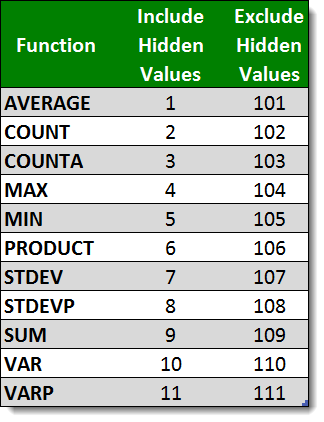
The function_num indicates which type of calculation you would like to perform. It has two sets of values. One- and two-digit values calculate only values that show in the filtered table, but they also include any manually hidden rows in the spreadsheet. Three-digit values indicate that SUBTOTAL should ignore both filtered rows and any rows that are manually hidden. In other words, with three-digit values, what you see is what you get.

A summary of the potential values of function_num is below:

In this example, we want the SUM calculation from SUBTOTAL. Since we are only dealing with filtered rows and not hidden rows, both 9 and 109 will work equally well. Let’s replace the calculations in the Total row.

Underneath the column for each year, type the SUBTOTAL function, indicate 9 for the function_num, and select the range of cells in the table for the corresponding year. The data table will convert that cell range (normally, D3:D28) to it’s Data Table range name. Repeat the process for each year’s column.

Re-filter the data, and you’ll find that the Total row re-calculates to provide the correct values! SUBTOTAL can just as easily be used to compute averages, find the maximum or minimum values among those on display, and more!