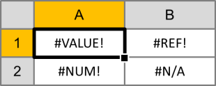
Excel functions like VLOOKUP, MATCH, and INDEX are great tools, but when they don’t work, they throw errors that can break an entire spreadsheet if referenced incorrectly. Error messages can be especially bad if they show up on end-user worksheets like reports and dashboards. Fortunately, Excel has a way to catch errors like #VALUE!, #NUM!, and #REF! before they show up. Learn how to handle error messages in Excel here…

Why Error Messages Appear

When you use functions in Excel, they expect their inputs to have certain characteristics. When you use SUM to add cells together, Excel assumes that the references are numbers. When you use VLOOKUP to find a value in cell range, Excel trusts that the value is there. Whenever Excel doesn’t find what it expects, it will return an error message.

Excel Error Types

#VALUE!

#VALUE! is likely the most common of errors. It occurs whenever the data type a function is given doesn’t match what it is expecting. A simple example would be adding a text value to a number:

="A"+1

#REF!

#REF! errors happen when a cell reference is deleted or moved. Excel tries to automatically update all references, but when it can’t do so, it replaces the actual cell reference with the error. For example, if we added the contents of cells A1 and B1, the function would look like this:

=A1+B1

After deleting cell B1, the function would revert to this:

=A1+#REF!

#DIV/0!

#DIV/0! happens when a mathematical operation attempts to divide by zero (which isn’t possible). Usually, this occurs because a COUNT or SUM results in zero and another cell is operating on its result. A simple example is dividing any number by zero:

=1/0

#NAME?

#NAME? appears when Excel can’t find a named range. Excel assumes that any un-quoted string that isn’t a function name is a named range. You will most likely encounter this when you forget to quote a string or mis-type a cell reference.  For example:

=A+1

#NULL!

#NULL! gets returned when Excel can’t figure out the range specified in a cell. This can happen when you put a space between function inputs instead of using a comma. For example:

=SUM(A1 C1)

#N/A

#N/A happens when a function like MATCH or VLOOKUP cannot find the value it is being asked to look for. For example:

=MATCH("A",{"B","C"},0)

False Errors in Excel

There are a couple of error conditions in Excel that aren’t true errors. They are usually a result of a formatting issue or a worksheet that is still calculating.

########

There are two reasons you could see a string of pound symbols (#) in a cell. The first is that the cell column is too narrow to display the value. The fix is simple: just expand the column to fit.

The second reason you could see ######## is if a date-formatted cell becomes negative. Usually this happens when times are subtracted. Because they hold a value close to zero (e.g. 6:00am is 0.25 on the number line), subtracting a small amount of time can bring the value negative. To learn more about how dates and times work in Excel, check out The Definitive Guide to Using Dates and Times in Excel.

In both cases, the data is still available in the cell – it is simply a formatting issue. Other formulas referencing the cell can still see and use the information, thus it isn’t a true error.

#GETTING_DATA

#GETTING_DATA is a message that can appear in Excel when a large or complex worksheet is being calculated. In Excel 2007 and newer, operations are grouped so more complicated cells may finish after earlier ones do. While the calculations are still processing, the unfinished cells may display #GETTING_DATA. Because the message is temporary and disappears when the calculations complete, this isn’t a true error.

Excel Error Handling Functions

Excel has a library of functions that can catch error messages before they are displayed. They can beautify a dashboard or report, and they can allow for nested lookup functions and more sophisticated worksheets.

ISNA

The ISNA function evaluates an #N/A error and returns a TRUE boolean. If the input isn’t an #N/A error, it returns FALSE. The syntax is as follows:

=ISNA(value)

ISERR

The ISERR function evaluates all error types except for #N/A. If the input is a #VALUE!, #REF!, #DIV/0, #NAME?, or #NULL! error, IFERR returns a TRUE boolean. If it is none of those error types, it returns FALSE. The syntax is as follows:

=ISERR(value)

ISERROR

The ISERROR function catches all error types and returns a TRUE boolean. If the input is a #VALUE!, #REF!, #DIV/0, #NAME?, #NULL! or #N/A error, it returns TRUE. If it is not an error, it returns FALSE. The syntax is as follows:

=ISERROR(value)

ERROR.TYPE

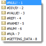
The ERROR.TYPE function will return a number from 1 through 8 that corresponds to the type of error in it’s input cell reference. If the cell reference doesn’t contain an error, the function returns it’s own #N/A error. The possible output values for ERROR.TYPE are as follows:

For example, if cell A1 contains a #VALUE! error:

=ERROR.TYPE(A1)

Returns 3 as a numeric value.

IFERROR

The IFERROR function combines the IF and ISERROR functions to allow an alternate function to be used if an error occurs. The syntax is as follows:

=IFERROR(value, value_if_error)

Common Error Handling Techniques

Catching Lookup Errors with IFERROR

When using VLOOKUP or HLOOKUP to fill fields from a lookup table, these functions will give an error if a match is not found. Rather than displaying an unsightly #VALUE!, IFERROR can catch the error and display an alternate message. Look at the following example:

=IFERROR(VLOOKUP(A1,C:C,1,FALSE),"No Match")

In the above formula, VLOOKUP is trying to find the contents of cell A1 in column C. If it cannot find a match, normally it would give an error, but instead it returns “No Match”.

Nested IFERROR Lookups

If a lookup like MATCH errors out on the first attempt, nested IFERROR functions can run a second or even a third lookup in its value_if_error field. Look at the following example:

=IFERROR(MATCH(A1,F2:F11,0),IFERROR(MATCH(A1,G:G,0),"No Match"))

In the above example, the first MATCH is trying to find the contents of cell A1 in the cells F2:F11. If it can’t find a match, normally it would return an error, but instead, we do another search for A1 in column G. Finally, if both MATCH functions, then the second IFERROR displays “No Match”.

Instructing Worksheet Users Through ISERROR

Error catches can also be used to instruct a user how to fill out forms or use a dashboard within a spreadsheet. Let’s say you have a calculation that divides by a cell that is user-input. The input must be non-zero, or the function won’t compute and a #DIV/0! error will be thrown. Next to the user-input cell, you can provide instructions based on their actions:

=IF(ISERROR(B5),”Value must be larger than zero.“,”Input accepted.“)

In this example, B5 is the calculation cell where the division happens. If the division operation throws a #DIV/0! error, the formula displays “Value must be larger than zero.” Otherwise, it just shows “Input accepted.“